Data Analytics Case Study — Bellabeat
Welcome to the Bellabeat Case Study. In this case study, I’ll be sharing how I used Data Analytics to help Bellabeat understand product usage trends to grow as a global company by shaping their marketing strategy.
Throughout this case study, I will use RStudio as my data analytics tool. I will also follow a structured data analysis process: Ask, Prepare, Process, Analyze, Share & Act. By adopting this methodology, I aim to uncover key insights into Bellabeat’s data-driven strategies.

ASK PHASE
Scenario
Bellabeat is a successful high-tech manufacturer of health-focused products for women, but they have the potential to become a larger player in the global smart device market. Urška Sršen, cofounder and Chief Creative Officer of Bellabeat, believes that analyzing smart device fitness data could help unlock new growth opportunities for the company. Therefore, my marketing analyst team needs to focus on one of Bellabeats’s products and analyze and undertand smart device data to gain insight into how consumers are using their smart devices. From these insights discovered, my team will then help guide marketing strategy for the company. My team will present our analysis to the Bellabeat executive team along with our high-level recommendations for Bellabeat’s marketing strategy.
By 2016, Bellabeat had opened offices around the world and launched multiple products. Bellabeat products became available through a growing number of online retailers in addition to their own e-commerce channel on their website. The company has invested in traditional advertising media, such as radio, out-of-home billboards, print, and television, but focuses on digital marketing extensively. Bellabeat invests year-round in Google Search, maintaining active Facebook and Instagram pages, and consistently engages consumers on Twitter. Additionally, Bellabeat runs video ads on Youtube and display ads on the Google Display Network to support campaigns around key marketing dates.
Sršen knows that an analysis of Bellabeat’s available consumer data would reveal more opportunities for growth. She has asked the marketing analytics team to focus on a Bellabeat product and analyze smart device usage data in order to gain insight into how people are already using their smart devices. Then, using this information, she would like high-level recommendations for how these trends can inform Bellabeat marketing strategy.
Problem: Bellabeat needs to expand and grow as a global health-focused smart product company.
Solution: Understand how clients are using their Bellabeat smart devices and uncover health trends.
Business Task/Purpose:
Analyze smart device usage data to identify trends and insights related to Bellabeat products in order to help inform and shape Bellabeat’s marketing strategy.
Stakeholders: Executive team members Urška Sršen and Sando Mur, and the Bellabeat marketing analytics team.
PREPARE PHASE
Data Sources:
FitBit Fitness Tracker Data from Mobius:
https://www.kaggle.com/arashnic/fitbit, which was generated from a distributed survey via Amazon Mechanical Turk. The dataset has 18 CSV files that contains recorded data from 30 participants, covering data from 04–11–2016 through 05–12–2016.
This is data that comes from the FitBit Fitness Tracker Data that was generated from a distributed survey via Amazon Mechanical Turk, so it’s objective, unbiased and credible. The data sources are also comprehensive, accurate and relevant to solve our business problem because they include all the factors that we need to analyzed smart device usage.
To evaluate the data’s credibility and integrity in detail, we can assess the most important data aspects:
- Reliable: The data is reliable because it’s from 30 FitBit users who consented to the submission of personal tracker data and generated from a distributed survey via Amazon Mechanical Turk.
- Original: The data is original because they’re real Fitbit users who consented to the submission of personal tracker data via Amazon Mechanical Turk.
- Comprehensive: The data is comprehensive for the most part because it has many factors like physical activity, sleep and calories recorded by date and time. However, the data contains a sample that only covers one month so it’s limited in this regard.
- Current: The data is not current because it’s from March 2016 to May 2016.
- Cited: The data is cited because we know it’s from the FitBit Fitness Tracker Data that was generated from a distributed survey via Amazon Mechanical Turk.
It’s important to address the data-privacy issues present and we can use it because the 30 FitBit users have consented to the submission of personal tracker data via Amazon Mechanical Turk.
These spreadsheets are organized in a wide format, where each row represents one specific record and the columns contain different attributes of the record, which include the minute-level output for physical activity, heart rate, steps taken and sleep monitoring, among others.
Installing packages needed for the analysis
Intalling the R packages and loading the libraries needed for our analysis.
#Installing the packages
install.packages('tidyverse')
install.packages('janitor')
install.packages('lubridate')
install.packages('skimr')

#Loading the packages
library(tidyverse)
library(janitor)
library(lubridate)
library(skimr)
library(ggplot2)
library(dplyr)
library(tidyr)
Loading the files
Creating 6 data frames with the most important and useful CSV files, by importing these files into R. I moved these the files to the folder ‘Fitbit Data’, inside my working directory:
#Loading our data
daily_activity <- read.csv("Fitbit Data/dailyActivity_merged.csv")
daily_sleep <- read.csv("Fitbit Data/sleepDay_merged.csv")
weight_log <- read.csv("Fitbit Data/weightLogInfo_merged.csv")
hourly_calories <- read.csv("Fitbit Data/hourlyCalories_merged.csv")
hourly_steps <- read.csv("Fitbit Data/hourlySteps_merged.csv")
minute_sleep <- read.csv("Fitbit Data/minuteSleep_merged.csv")
hourly_heartrate <- read.csv("Fitbit Data/heartrate_seconds_merged.csv")
Then, we can inspect our data to see the structure of the data frames:
str(daily_activity)
str(daily_sleep)
str(weight_log)
str(hourly_calories)
str(hourly_steps)
str(minute_sleep)
str(hourly_heartrate)
PROCESS PHASE
Cleaning the column names
Changing the column names to snake_case for all the data frames:
daily_activity <- clean_names(daily_activity)
daily_sleep <- clean_names(daily_sleep)
weight_log <- clean_names(weight_log)
hourly_calories <- clean_names(hourly_calories)
hourly_steps <- clean_names(hourly_steps)
minute_sleep <- clean_names(minute_sleep)
hourly_heartrate <- clean_names(hourly_heartrate)
Changing the data formats
After inspecting our data we see that the dates of all the data frames have the format character, so we change them to a date and date time format:
daily_activity$activity_date <- as.Date(daily_activity$activity_date,"%m/%d/%Y")
daily_sleep$sleep_day <- as.Date(daily_sleep$sleep_day, '%m/%d/%Y')
weight_log$date <- parse_date_time(weight_log$date, '%m/%d/%Y %H:%M:%S %p')
weight_log$is_manual_report <- as.logical(weight_log$is_manual_report)
hourly_calories$activity_hour <- parse_date_time(hourly_calories$activity_hour, '%m/%d/%Y %H:%M:%S %p')
hourly_steps$activity_hour <- parse_date_time(hourly_steps$activity_hour, '%m/%d/%Y %H:%M:%S %p')
minute_sleep$date <- parse_date_time(minute_sleep$date, '%m/%d/%Y %H:%M:%S %p')
hourly_heartrate$time <- mdy_hms(hourly_heartrate$time)
hourly_heartrate$time <- format(hourly_heartrate$time, "%Y-%m-%d %H:%M:%S")
Checking for duplicated rows and deleting them
We check for duplicated data so we can delete them:
#Check for duplicated rows and delete them
sum(duplicated(daily_activity))
sum(duplicated(daily_sleep))
daily_sleep <- daily_sleep[!duplicated(daily_sleep), ]
sum(duplicated(weight_log))
sum(duplicated(hourly_calories))
sum(duplicated(hourly_steps))
sum(duplicated(minute_sleep))
minute_sleep <- minute_sleep[!duplicated(minute_sleep), ]
sum(duplicated(hourly_heartrate))
Checking for missing data
We’ll check for missing data in all the data frames.
#Checking for missing data
dim(daily_sleep)
sum(is.na(daily_sleep))
sum(is.na(daily_activity))
sum(is.na(weight_log))
sum(is.na(hourly_calories))
sum(is.na(hourly_steps))
sum(is.na(minute_sleep))
sum(is.na(hourly_heartrate))
Removing the column fat
The only table that has missing data is the weight_log dataframe. I will remove the column fat since almost all values are missing.
weight_log <- weight_log %>%
  select(-c(fat))
Adding Columns
Important columns for analysis will be added to all the data frames. The columns dates and hour will be added to make the table joining/merging process easier later.
Adding columns to the daily_activity data frame
Adding columns day_of_week, total_active_hours, sedentary_hours and dates to the daily_activity data frame. Also adding columns total_minutes, sedentary_percentage, lightly_percentage, fairly_percentage and very_active_percentage:
#Adding columns to the daily_activity dataframe
daily_activity$day_of_week <- wday(daily_activity$activity_date, label = T, abbr = T)
daily_activity$total_active_hours = round((daily_activity$very_active_minutes + daily_activity$fairly_active_minutes + daily_activity$lightly_active_minutes)/60, digits = 2)
daily_activity$sedentary_hours = round((daily_activity$sedentary_minutes)/60, digits = 2)
daily_activity$dates <- daily_activity$activity_date

daily_activity$total_minutes <- daily_activity$very_active_minutes + daily_activity$fairly_active_minutes + daily_activity$lightly_active_minutes + daily_activity$sedentary_minutes
daily_activity$sedentary_percentage <- round(daily_activity$sedentary_minutes / daily_activity$total_minutes, 4)
daily_activity$lightly_percentage <- round(daily_activity$lightly_active_minutes / daily_activity$total_minutes, 4)
daily_activity$fairly_percentage <- round(daily_activity$fairly_active_minutes / daily_activity$total_minutes, 4)
daily_activity$very_active_percentage <- round(daily_activity$very_active_minutes / daily_activity$total_minutes, 4)
Adding columns to the daily_sleep data frame
Adding columns day_of_week, hours_in_bed, hours_asleep, time_taken_to_sleep, time_taken_to_sleep_percentage and dates to the daily_sleep data frame.
#Adding columns to the daily_sleep dataframe
daily_sleep$day_of_week <- wday(daily_sleep$sleep_day, label = T, abbr = T)
daily_sleep$hours_in_bed = round((daily_sleep$total_time_in_bed)/60, digits = 2)
daily_sleep$hours_asleep = round((daily_sleep$total_minutes_asleep)/60, digits = 2)
daily_sleep$time_taken_to_sleep = (daily_sleep$total_time_in_bed - daily_sleep$total_minutes_asleep)
daily_sleep$time_taken_to_sleep_percentage <- round(daily_sleep$time_taken_to_sleep/daily_sleep$total_time_in_bed, 4)
daily_sleep$dates <- daily_sleep$sleep_dayr
Adding columns to the weight_log data frame
Adding columns bmi2, hour and dates to the weight_log data frame. The column bmi2 will be created based on the categories ‘Overweight’, ‘Healthy’ and ‘Underweight’, according to their values.
weight_log <- weight_log %>%
  mutate(bmi2 = case_when(
    bmi > 24.9 ~ 'Overweight',
    bmi < 18.5 ~ 'Underweight',
    TRUE ~ 'Healthy'
  ))
weight_log$hour <- hour(weight_log$date)
weight_log$dates <- date(weight_log$date)
Adding columns to the hourly data frames
Adding columns hour and dates to the hourly_calories, hourly_steps, minute_sleep and hourly_heartrate data frames.
#Adding columns to the hourly_calories dataframe
hourly_calories$hour <- hour(hourly_calories$activity_hour)
hourly_calories$dates <- date(hourly_calories$activity_hour)

#Adding columns to the hourly_steps dataframe
hourly_steps$hour <- hour(hourly_steps$activity_hour)
hourly_steps$dates <- date(hourly_steps$activity_hour)

#Adding columns to the minute_sleep dataframe
minute_sleep$hour <- hour(minute_sleep$date)
minute_sleep$dates <- date(minute_sleep$date)
minute_sleep$day_of_week <- wday(minute_sleep$dates, label = T, abbr = T)

#Adding columns to the hourly_heartrate dataframe
hourly_heartrate$hour <- hour(hourly_heartrate$time)
hourly_heartrate$dates <- as.Date(hourly_heartrate$time)
Removing inconsistent data rows
Burning 0 or less calories per day is impossible, therefore these rows will be removed. Total active hours of 0 or less aren’t possible either since it’s expected that users at least get out of bed:
#Remove rows to clean data
daily_activity <- daily_activity[!(daily_activity$calories<=0),]
daily_activity <- daily_activity[!(daily_activity$total_active_hours<=0.00),]
hourly_calories <- hourly_calories[!(hourly_calories$calories<=0),]
Merging all the data frames
Merging the data frames into merged_data and hourly_weight:
#Merging the dataframes
#Merging to get hourly_weight
hourly_steps_calories <- merge(hourly_calories, hourly_steps, by=c("id", "dates", "hour"), all=TRUE)
hourly_weight <- merge(hourly_steps_calories, weight_log, by=c("id", "dates", "hour"), all=TRUE)

#Merging the 3 main data frames
activity_weight <- merge(daily_activity, weight_log, by=c("id", "dates"), all=TRUE)
merged_data <- merge(activity_weight, daily_sleep, by=c("id", "dates"), all=TRUE)
Exporting our data
#Exporting our cleaned data
write.csv(daily_activity, file ='fitbit_daily_activity.csv')
write.csv(daily_sleep, file = 'fitbit_sleep_log.csv')
write.csv(weight_log, file = 'fitbit_weight_log.csv')
write.csv(hourly_calories, file = 'fitbit_hourly_calories.csv')
write.csv(hourly_steps, file = 'fitbit_hourly_steps.csv')
write.csv(minute_sleep, file = 'fitbit_minute_sleep.csv')
write.csv(hourly_heartrate, file = 'fitbit_hourly_heartrate.csv')

write.csv(hourly_weight, file = 'fitbit_hourly_weight.csv')
hourly_weight <- read.csv('fitbit_hourly_weight.csv')

write.csv(merged_data, file = 'fitbit_merged_data.csv')
merged_data <- read.csv('fitbit_merged_data.csv')
Data Cleaning Documentation
Change Log
Version 4.0.0 (07–07–2023)
New
- The R program was selected for its high functionality at cleaning data. Created 6 data frames while importing CSV files into R, with names daily_activity, daily_sleep, weight_log, hourly_calories, hourly_steps, minute_sleep and hourly_heartrate.
- Added columns day_of_week, total_active_hours, sedentary_hours and dates to the daily_activity data frame.
- Added columns columns total_minutes, sedentary_percentage, lightly_percentage, fairly_percentage and very_active_percentage to the daily_activity data frame.
- Added columns day_of_week, hours_in_bed, hours_asleep, time_taken_to_sleep, time_taken_to_sleep_percentage and dates to the daily_sleep data frame.
- Added columns bmi2, hour and dates to the weight_log data frame.
- Added columns hour and dates to the hourly_calories data frame.
- Added columns hour and dates to the hourly_steps data frame.
- Added columns hour, dates and day_of_week to the minute_sleep data frame.
- Added columns hour and dates to the hourly_heartrate data frame.
- Created the data frame merged_data to join/merge all the previous data frames and export the data cleaned up and prepared for analysis to other tools like spreadsheets and Tableau.
Changes
- Changed the name of all the columns to snake_case for all the data frames.
- Changed the format of the dates from all the data frames from character to date or date time.
- Changed the format of the column is_manual_report from character to logical.
Removed
- Removed duplicated data rows from daily_sleep.
- Removed duplicated data rows from minute_sleep.
- Removed the column fat from the weight_log data frame.
- Removed data rows from daily_activity and hourly_calories where the number of calories burned per day are 0 or less.
- Removed data rows from daily_activity where the total active hours are 0 or less.
After these steps it’s confirmed that the data is integral, clean and ready to analyze.
ANALYZE AND SHARE PHASES
Analyzing and Visualizing Data
Summary Statistics
First we’re going to analyze summary statistics to extract some general insights:
#Summary Statistics
> summary(merged_data$total_steps)   Min. 1st Qu.  Median    Mean 3rd Qu.    Max.
      0    4920    8053    8319   11100   36019
> summary(merged_data$sedentary_hours)
   Min. 1st Qu.  Median    Mean 3rd Qu.    Max.
   0.00   12.02   17.00   15.87   19.80   23.98
> summary(merged_data$sedentary_percentage)
   Min. 1st Qu.  Median    Mean 3rd Qu.    Max.
 0.0000  0.7229  0.7771  0.7805  0.8465  0.9993> summary(merged_data$very_active_minutes)
   Min. 1st Qu.  Median    Mean 3rd Qu.    Max.
   0.00    0.00    7.00   23.21   36.00  210.00> summary(merged_data$fairly_active_minutes)
   Min. 1st Qu.  Median    Mean 3rd Qu.    Max.
   0.00    0.00    8.00   14.88   21.00  143.00
> summary(merged_data$lightly_active_minutes/60)
   Min. 1st Qu.  Median    Mean 3rd Qu.    Max.
  0.000   2.467   3.483   3.525   4.533   8.633
> summary(merged_data$hours_asleep)
   Min. 1st Qu.  Median    Mean 3rd Qu.    Max.    NA's
  0.970   6.020   7.210   6.987   8.170  13.270     447
> summary(merged_data$time_taken_to_sleep)
   Min. 1st Qu.  Median    Mean 3rd Qu.    Max.    NA's
   0.00   17.00   25.50   39.31   40.00  371.00     447
> summary(merged_data$time_taken_to_sleep_percentage)
   Min. 1st Qu.  Median    Mean 3rd Qu.    Max.    NA's
 0.0000  0.0394  0.0574  0.0835  0.0882  0.5016     447
> summary(merged_data$total_active_hours)
   Min. 1st Qu.  Median    Mean 3rd Qu.    Max.
   0.02    3.08    4.30    4.16    5.38    9.20
> summary(merged_data$weight_kg)
   Min. 1st Qu.  Median    Mean 3rd Qu.    Max.    NA's
  52.60   61.40   62.50   72.04   85.05  133.50     790
> summary(merged_data$calories)
   Min. 1st Qu.  Median    Mean 3rd Qu.    Max.
     52    1854    2218    2359    2830    4900
#Alternatively all variables at the same time
summary(merged_data)- The average number of steps per day is 8319, which is below the recommended aim of 10,000 steps for adults.
- The average sedentary hours per day are 15.87 hours, which is 78.05% of their daily time and below the limit of 10 hours at most.
- The average very active time per day is 23.21 minutes, which is 2.02% of their daily time and above the recommended time of 10.71 minutes of vigorous exercise per day.
- The average fairly active time per day is 14.88 minutes, which is 1.31% of their daily time and above the recommended time of 21.43 minutes of moderate intensity activity per day.
- The average lightly active time per day is 3.5 hours, which is 18.63% of their daily time and above the recommended time of 30 minutes per day of light intense activity like walking and household chores.
- The avegage time being asleep is 6.987 hours, which almost reaches the recommended time of 7–9 hours.
- The average time take to sleep is 39.31 minutes, which represents the 8.35% of time being in bed.
- The average time of being at least a little active is 4.16 hours.
- The average weight is 72.04 kg, but we only have this data for 8 people.
- The average burned calories per day is 2359, which surpass the recommended amount of 2,000 for women.
Analyzing the Distribution of the data
We’re going to create histograms to analyze the distribution of the data:
#Distribution of data
ggplot(data = merged_data, aes(x = total_steps)) +
  geom_histogram(binwidth = 2000, fill='lightblue') +
  labs(x = 'Total Steps per Day', y = 'Frequency', title = 'Distribution of Daily Total Steps') +
  scale_x_continuous(breaks = seq(min(merged_data$total_steps), max(merged_data$total_steps), by = 4000))

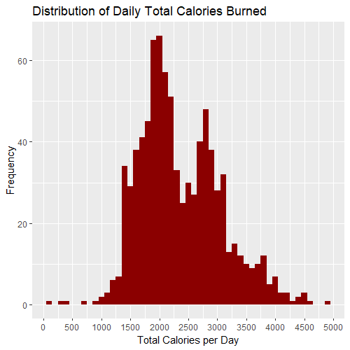
ggplot(data = merged_data, aes(x = calories)) +
  geom_histogram(binwidth = 100, fill='darkred') +
  labs(x = 'Total Calories per Day', y = 'Frequency', title = 'Distribution of Daily Total Calories Burned') +
  scale_x_continuous(breaks = seq(min(0), max(7000), by = 500))

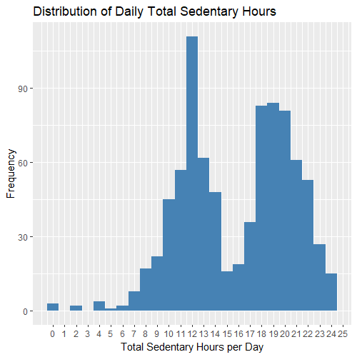
ggplot(data = merged_data, aes(x = sedentary_hours)) +
  geom_histogram(binwidth = 1.00, fill='steelblue', na.rm = FALSE) +
  labs(x = 'Total Sedentary Hours per Day', y = 'Frequency', title = 'Distribution of Daily Total Sedentary Hours') +
  scale_x_continuous(breaks = seq(min(0.00), max(25.00), by = 1.00))

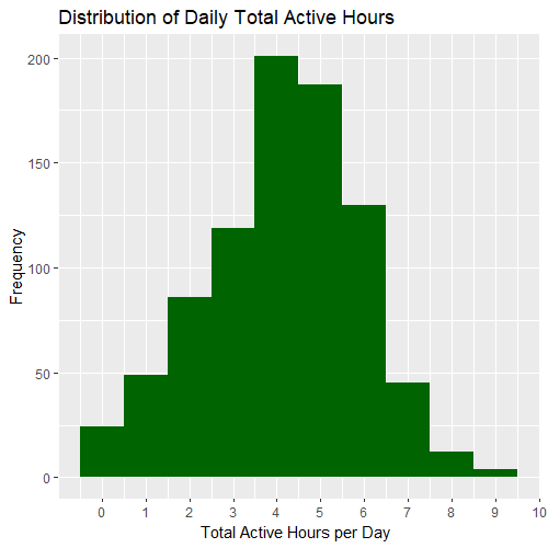
ggplot(data = merged_data, aes(x = total_active_hours)) +
  geom_histogram(binwidth = 1.00, fill='darkgreen', na.rm = FALSE) +
  labs(x = 'Total Active Hours per Day ', y = 'Frequency', title = 'Distribution of Daily Total Active Hours') +
  scale_x_continuous(breaks = seq(min(0.00), max(10.00), by = 1.00))

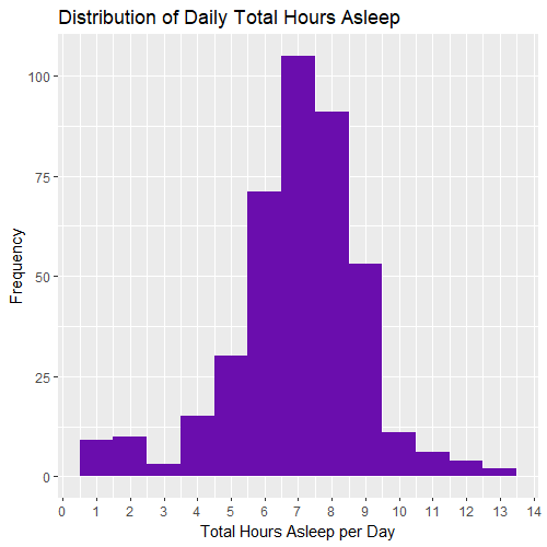
ggplot(data = merged_data, aes(x = hours_asleep)) +
  geom_histogram(binwidth = 1.00, fill='#6A0DAD', na.rm = FALSE) +
  labs(x = 'Total Hours Asleep per Day', y = 'Frequency', title = 'Distribution of Daily Total Hours Asleep') +
  scale_x_continuous(breaks = seq(min(0.00), max(14.00), by = 1.00))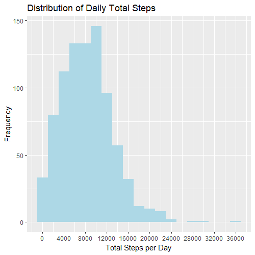
- The number of steps taken per day that are recorded with most frequency are between 5000 and 11000 steps, which represents 54% of all days (this was taken from Tableau when displaying the percentages). This means that most users mostly take a number of steps inside that range per day.
- Most users burn most calories per day between 1700 and 2100 calories (32% of days) and between 2500 and 2900 calories (21% of days).
- Most users spend either around 11–12 (19% of days) or between 17 and 20 sedentary hours per day (32% of days), which is very high, but we have to remember that in this dataset sedentary hours include hours asleep.
- Most users mostly spend a number of total active hours per day between 3.5 and 5.5 hours, which represents 44% of all days.
- The number of total hours asleep per day that are recorded with most frequency are between 5.5 and 8.5 hours (71% of of all days).
Analyzing daily activity
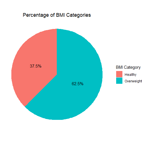
Creating a pie chart for active and sedentary minutes, and for BMI of the users. We also want to know how many weight data we have so we can plot a pie chart of the BMI of the users:
#Creating pie charts
total_minutes <- sum(daily_activity$very_active_minutes, daily_activity$fairly_active_minutes, daily_activity$lightly_active_minutes, daily_activity$sedentary_minutes)

very_active_percentage <- round((sum(daily_activity$very_active_minutes) / total_minutes) * 100, 2)
fairly_percentage <- round((sum(daily_activity$fairly_active_minutes) / total_minutes) * 100, 2)
lightly_percentage <- round((sum(daily_activity$lightly_active_minutes) / total_minutes) * 100, 2)
sedentary_percentage <- round((sum(daily_activity$sedentary_minutes) / total_minutes) * 100, 2)

data <- data.frame(Activity = c("Very Active", "Fairly Active", "Lightly Active", "Sedentary"),
                   Percentage = c(very_active_percentage, fairly_percentage, lightly_percentage, sedentary_percentage))

pie_chart <- ggplot(data, aes(x = "", y = Percentage, fill = Activity)) +
  geom_bar(width = 1, stat = "identity") +
  coord_polar("y", start = 0) +
  theme_void() +
  labs(fill = "Activity Type", title = "Percentage of Activity Types") +
  scale_fill_manual(values = rainbow(length(data$Activity))) +
  geom_text(aes(label = paste0(Percentage, "%")),
            position = position_stack(vjust = 0.6),
            position_stack = 1,
            angle = 0,
            color = "black") +
  theme(legend.position = "right",
        plot.title = element_text(hjust = 0.5))

print(pie_chart)

#Descriptive analysis
#The amount of healthy users
> nrow(filter(distinct(weight_log, id, .keep_all = T),bmi2 == 'Healthy'))
[1] 3
#The amount of underweight users
> nrow(filter(distinct(weight_log, id, .keep_all = T),bmi2 == 'Underweight'))
[1] 0
#The amount of overweight users
> nrow(filter(distinct(weight_log, id, .keep_all = T),bmi2 == 'Overweight'))
[1] 5
#Creating a pie chart with BMI categories for the users
summary_table <- weight_log %>%
  distinct(id, bmi2) %>%
  count(bmi2) %>%
  mutate(percentage = n / sum(n) * 100)

ggplot(summary_table, aes(x = "", y = percentage, fill = bmi2)) +
  geom_bar(stat = "identity", width = 1) +
  coord_polar("y", start = 0) +
  theme_void() +
  labs(fill = "BMI Category", title = "Percentage of BMI Categories") +
  geom_text(aes(label = ifelse(percentage != 0, paste0(round(percentage, 1), "%"), "")), position = position_stack(vjust = 0.5)) +
  theme(plot.title = element_text(hjust = 0.5))
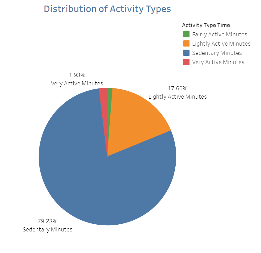
- On average, the users spend most part of their daily activity being sedentary (81.33%), while 15.82% of their time they engage in lighty activity; this tells us that they need to engage in more active activities to be healthier.
- We only have weight data for 8 users; 5 of them (62.5%) are overweight and the other 3 users (37.5%) are healthy.
Now we want to know if they are reaching the recommended quota of moderate and intense activity. It’s recommended by the Centers for Disease Control and Prevention (CDC) that people do at least 150 minutes of moderate intensity activity a week or 75 minutes of vigorous intensity activity a week. This means that people need to do 21.43 minutes being fairly active per day or 10.71 minutes being very active.
active_people <- daily_activity %>%
  filter(fairly_active_minutes >= 21.4 | very_active_minutes>=10.7) %>%
  group_by(id) %>%
  count(id)
print(active_people)
view(active_people)
> summary(active_people) Min.   :1.504e+09   Min.   : 1.00
 1st Qu.:2.998e+09   1st Qu.: 6.25
 Median :4.631e+09   Median :15.50
 Mean   :5.079e+09   Mean   :15.23
 3rd Qu.:6.996e+09   3rd Qu.:22.75
Max. :8.878e+09 Max. :30.00 - Here we can see that, on average, people reach this quota for 15.23 days of the evaluated period. This means that the users are active only half the days within the entire month.
Now we want to know how many users manage to do the recommended quota of moderate and intense activity for the recommeded 22 days or more in a month.
active_people_surpassing_22 <- daily_activity %>%
  filter(fairly_active_minutes >= 21.4 | very_active_minutes >= 10.7) %>%
  group_by(id) %>%
  count() %>%
  filter(n >= 22)

n_ids_surpassing_22 <- sum(active_people_surpassing_22$n > 22)
> print(n_ids_surpassing_22)
[1] 8- Only 8 users out of 30 (26.67%) manage to reach the recommended quota of moderate and intense activity for the recommeded 22 days or more in a month. This suggests that since the averages above were mostly positive, people who engage in more physical activities are influencing this average by exceeding the healthy quota by a substantial amount, while most users (73.33%) aren’t active enough to be healthy.
Activity data by Day of the Week
Now we’re going to analyze activity data by day of the week, making more key visualizations to draw important insights:
#Visualizing activity per day of the week
options(scipen = 999)
ggplot(data = merged_data) +
  aes(x = day_of_week.x, y = total_steps) +
  geom_col(fill =  'darkgreen') +
  labs(x = 'Day of Week', y = 'Total Steps', title = 'Total Steps taken by Day of the Week')

ggplot(data = merged_data) +
  aes(x = day_of_week.x, y = total_active_hours) +
  geom_col(fill =  'brown') +
  labs(x = 'Day of Week', y = 'Total Active Hours', title = 'Total Active Hours by Day of the Week')

ggplot(data = daily_activity) +
  aes(x = day_of_week, y = calories) +
  geom_col(fill =  'red') +
  labs(x = 'Day of Week', y = 'Total Calories Burned', title = 'Total Calories Burned by Day of the Week')

ggplot(data = daily_activity) +
  aes(x = day_of_week, y = sedentary_hours) +
  geom_col(fill =  'blue') +
  labs(x = 'Day of Week', y = 'Total Sedentary Hours', title = 'Total Sedentary Hours by Day of the Week')

#Minutes per Day of Week
daily_activity_long_minutes <- pivot_longer(daily_activity, cols = c(very_active_minutes, fairly_active_minutes, lightly_active_minutes, sedentary_minutes),
                                            names_to = "MinutesType", values_to = "Minutes")

category_order_minutes <- c("very_active_minutes", "fairly_active_minutes", "lightly_active_minutes", "sedentary_minutes")

ggplot(daily_activity_long_minutes, aes(x = factor(day_of_week), y = Minutes, fill = factor(MinutesType, levels = category_order_minutes))) +
  geom_bar(stat = "identity", position = "dodge") +
  labs(x = "Day of Week", y = "Minutes", title = "Minutes by Day of Week", fill = "Activity Type Time") +
  scale_x_discrete(labels = c("Sun", "Mon", "Tue", "Wed", "Thu", "Fri", "Sat")) +
  scale_fill_manual(values = c("very_active_minutes" = "lightgreen", "fairly_active_minutes" = "yellow",
                               "lightly_active_minutes" = "orange", "sedentary_minutes" = "steelblue"),
                    labels = c("Very Active Minutes", "Fairly Active Minutes", "Lightly Active Minutes", "Sedentary Minutes"),
                    breaks = category_order_minutes) +
  theme_minimal()

#Miles per Day of Week
daily_activity_long_distance <- pivot_longer(daily_activity, cols = c(very_active_distance, moderately_active_distance, light_active_distance),
                                             names_to = "DistanceType", values_to = "Miles")


category_order_distance <- c("very_active_distance", "moderately_active_distance", "light_active_distance")

ggplot(daily_activity_long_distance, aes(x = factor(day_of_week), y = Miles, fill = factor(DistanceType, levels = category_order_distance))) +
  geom_bar(stat = "identity", position = "dodge") +
  labs(x = "Day of Week", y = "Miles", title = "Miles by Day of Week", fill = "Activity Type Distance") +
  scale_x_discrete(labels = c("Sun", "Mon", "Tue", "Wed", "Thu", "Fri", "Sat")) +
  scale_fill_manual(values = c("very_active_distance" = "purple", "moderately_active_distance" = "steelblue",
                               "light_active_distance" = "darkred"),
                    labels = c("Light Active Distance", "Moderately Active Distance", "Very Active Distance"),
                    breaks = category_order_distance) +
  theme_minimal()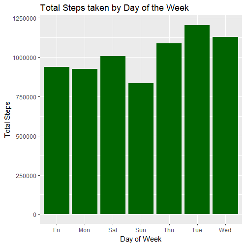
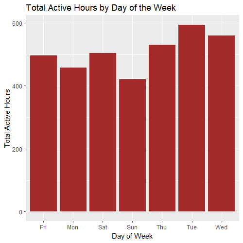
- Users are more active and take more steps on mid weekdays, mainly on Tuesdays, Wednesdays and Thursdays. However, they are more active and take more steps on Saturdays than on Mondays or Fridays, with Sundays being the less active days.
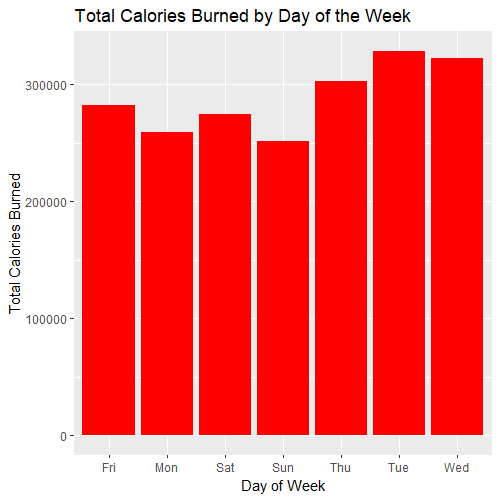
- For calories burned the pattern is the same except that users burn more calories on Fridays than on Saturdays.
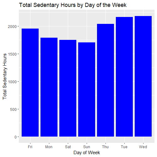
- Users also spend more time with sedentary activities on the weekdays from Tuesdays to Fridays and spend less time being sedentary on the weekends and on Mondays.
- Users are less active, take less steps and spend less calories on Sundays, but interestingly, they also spend the least time in sedentary activities on Sundays.
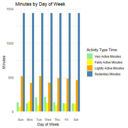
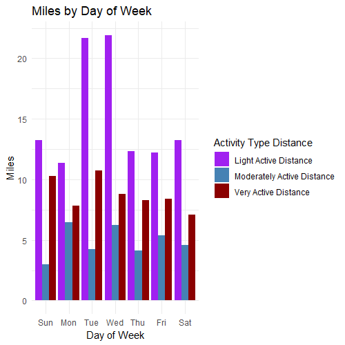
- Users cover more miles when they do light activities and the least when they do moderate-intensity activities.
From this we can conclude:
- Although involved in work and school activities for the most part of the day, users tend to prioritize doing physical activities during mid-weekdays Tuesdays, Wednesdays and Thursdays. The fact that Mondays and Fridays don’t show such tendency supports this conclusion because it means that only commuting to work and doing day-to-day (weekday) activities are not the main factor for the increased exercise on mid-weekdays. This tells us that users are more motivated to do physical activity in the middle of the week.
- Similarly, users are less active on Sundays, but also spend less time in sedentary activities. This might be a result of not doing work activities but also not doing much physical exercise since most users prefer to relax on Sundays.
- Users cover more miles when they’re lightly active. This is because, as we were expecting, lightly active activities mainly involve exercises that include walking, while when users do moderate and vigorous exercises, they probably don’t get involved much in cardio exercises but mainly in lifting weights and strength training exercises. Since both of these intensities involve roughly the same amount of time doing cardio exercises, it was expected that the most intense activities cover more miles than the moderately-intensity activities because more intensity usually involves running faster in these types of exercises.
- Users do light activities that cover the most miles on Tuesdays and Wednesdays, which reinforces the idea that users do more activities that involve walking these days. We can also see that users do more intense activities that cover the most miles on Tuesdays, Wednesdays and Saturdays, which is in harmony with what we dicovered before.
Activity and Sleep per Hour of the Day
Now we’re going to analyze the activity per hour of the day and sleep per hour and day of the week.
#Hourly Activity
options(scipen = 999)
ggplot(data = hourly_steps, aes(x = hour, y = step_total, fill = hour)) +
  geom_bar(stat = "identity") +
  labs(x = 'Hour of the Day', y = 'Total Steps Taken', title = "Hourly Distribution of Steps Taken") +
  scale_x_continuous(breaks = unique(hourly_steps$hour)) +
  scale_fill_gradient(name= 'Hours', low = "lightblue", high = "steelblue")

ggplot(data = hourly_calories, aes(x = hour, y = calories, fill = hour)) +
  geom_bar(stat = "identity") +
  labs(x = 'Hour of the Day', y = 'Calories Burned', title = "Hourly Distribution of Calories Burned") +
  scale_x_continuous(breaks = unique(hourly_calories$hour)) +
  scale_fill_gradient(name= 'Hours', low = "lightcoral", high = "darkred")

ggplot(data = hourly_heartrate, aes(x = hour, y = value, fill = hour)) +
  geom_bar(stat = "identity") +
  labs(x = 'Hour of the Day', y = 'Sum of Heart Rate Values', title = "Hourly Distribution of Total Heart Rate Values") +
  scale_x_continuous(breaks = unique(hourly_heartrate$hour)) +
  scale_fill_gradient(name= 'Hours', low = "lightgreen", high = "darkgreen")

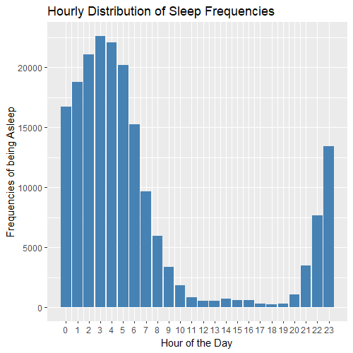
ggplot(data = minute_sleep, aes(x = hour)) +
  geom_bar(fill = "steelblue") +
  labs(x = 'Hour of the Day', y = 'Frequencies of being Asleep', title = "Hourly Distribution of Sleep Frequencies") +
  scale_x_continuous(breaks = unique(minute_sleep$hour))

#Sleep by Hour of the Day and Day of Week
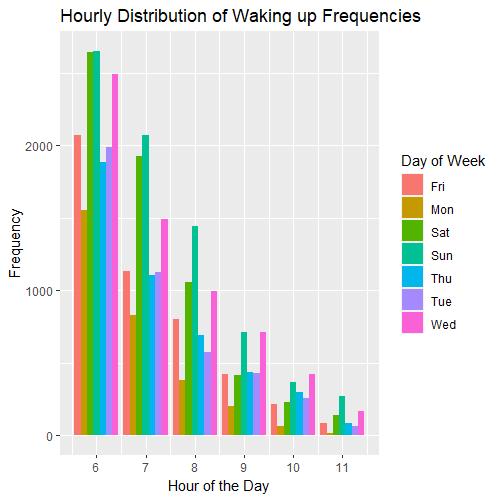
filtered_wake <- minute_sleep %>%
  filter(hour >= 6 & hour <= 11)

ggplot(filtered_wake, aes(x = hour, fill = day_of_week)) +
  geom_bar(position="dodge") +
  scale_x_continuous(breaks = 6:11) +
  labs(x = "Hour of the Day", y = "Frequency", title = "Hourly Distribution of Waking up Frequencies") +
  scale_fill_discrete(name = "Day of Week")

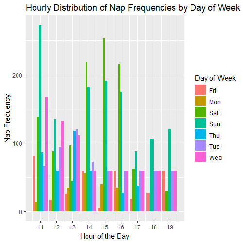
filtered_naps <- minute_sleep %>%
  filter(hour >= 11 & hour <= 19)

ggplot(filtered_naps, aes(x = hour, fill = day_of_week)) +
  geom_bar(stat = "count", position="dodge") +
  scale_x_continuous(breaks = 11:19) +
  labs(x = "Hour of the Day", y = "Nap Frequency", title = "Hourly Distribution of Nap Frequencies by Day of Week") +
  scale_fill_discrete(name = "Day of Week")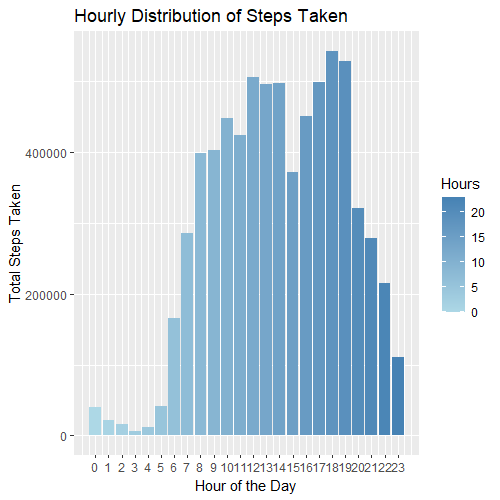
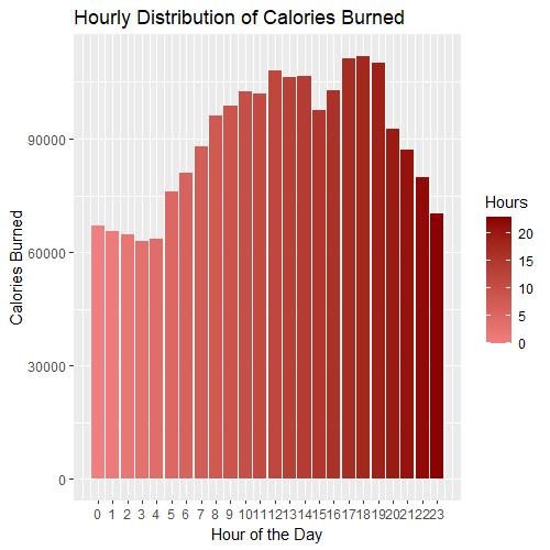
- The amount of steps taken and calories burned per hour of the day show a similar pattern. Most steps and most calories are expended between 12:00 and 15:00 hours, and between 17:00 and 20:00 hours. This tells us that most users
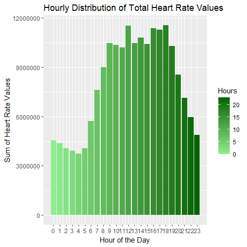
- The highest heart rate values take place between 12:00 and 13:00 hours, and between 16:00 and 19:00 hours, which is similar to the pattern found for calories and steps.
- This suggests that most calories spent at midday (from 12:00 to 14:30 hours) are burned from walking and typical day-to-day activities like going for lunch and returning to the office; and the calories spent after work in the early evening and evening (from 17:00 to 19:30 hours) are probably divided between returning from work activities and exercising.
- Most users start sleeping between 23:00 and 00:00 hours and wake up between 7:00 and 8:00 hours. It’s recommended that people sleep from 22:00/23:00 to 6:00/7:00 hours but only 4% of the days, users go to sleep at that time while still getting up early, since only 5% of the days users are waking up from 7:00 to 8:00 hours.
- We can see that many users are stil asleep at 8, 9, 10 and 11 AM on Sundays and Saturdays, so users wake up later these days, and Mondays are the days when people wake up the earliest. This suggests that most users change their sleep schedule on the weekends to sleep more and adjusting this for the start of the working days (Mondays) is difficult for most people.
- We can see that, in general, users also tend to take naps. The nap time constitutes 4.11% of the total time being asleep, which is 17.23 minutes per day on average.
- The most common time to take naps are between 12:00 and 13:59 hours on weedays and between 14:00 and 16:59 hours on the weekends. Users the most naps on the weekends, followed by Wednesdays and Tuesdays. Users take much fewer naps on Mondays and Fridays. This suggests that naps are taken when people have the time to rest and recover, since Mondays are the busiest days and Fridays are often spent to go out with friends.
Relationships
Now we’re going to analyze correlations between key factors:
#Relationships
ggplot(data = daily_activity) +
  aes(x= total_active_hours, y = calories) +
  geom_point(color = 'red') +
  geom_smooth() +
  labs(x = 'Total Active hours', y = 'Calories Burned', title = 'Calories Burned vs Active Hours')

ggplot(data = daily_activity) +
  aes(x= total_steps, y = calories) +
  geom_point(color = 'orange') +
  geom_smooth() +
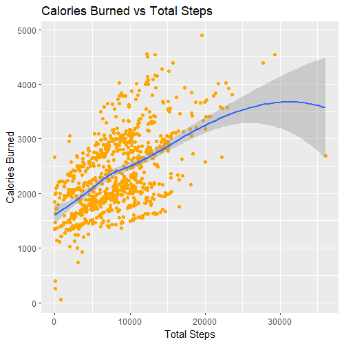
  labs(x = 'Total Steps', y = 'Calories Burned', title = 'Calories Burned vs Total Steps')

ggplot(data = daily_activity) +
  aes(x= sedentary_hours, y = calories) +
  geom_point(color = 'steelblue') +
  geom_smooth() +
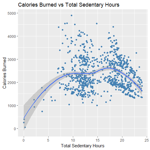
  labs(x = 'Total Sedentary Hours', y = 'Calories Burned', title = 'Calories Burned vs Total Sedentary Hours')

#Plotting weight against activity
sum_total_active <- merged_data %>%
  group_by(weight_kg) %>%
  summarise(sum_total_active_hours = sum(total_active_hours))

ggplot(data = sum_total_active) +
  aes(x = weight_kg, y = sum_total_active_hours) +
  geom_point(color = 'darkgreen') +
  geom_line(color = 'darkgreen') +
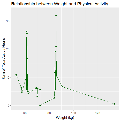
  labs(x = 'Weight (kg)', y = 'Sum of Total Active Hours', title = 'Relationship between Weight and Physical Activity') +
  scale_y_continuous(limits = c(0, 33))


sum_total_steps <- merged_data %>%
  group_by(weight_kg) %>%
  summarise(sum_total_steps = sum(total_steps))

options(scipen = 999)
ggplot(data = sum_total_steps) +
  aes(x = weight_kg, y = sum_total_steps) +
  geom_point(color = 'blue') +
  geom_line(color = 'blue') +
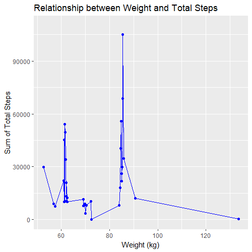
  labs(x = 'Weight (kg)', y = 'Sum of Total Steps', title = 'Relationship between Weight and Total Steps')+
  scale_y_continuous(limits = c(0, 110000))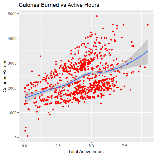
- There’s a positive correlation between the calories burned and the total active hours.
- There’s a positive correlation between the calories burned and the total steps taken.
- There’s isn’t a significative correlation between the calories burned and the total sedentary hours. This might be because in the data we have, sendentary hours also include hours asleep. As sleep patterns vary among individuals, it influences the overall sedentary time and diminishes the correlation with calorie burn.
- The most active users are 62 and 85 kg.
We can also investigate other obvious facts by plotting the relationship between total steps and total active and sedentary time.
#Relationship between Total Steps per Day and Activity Hours
ggplot(merged_data, aes(x = total_steps)) +
  geom_point(aes(y = sedentary_hours, color = "Sedentary Time")) +
  geom_point(aes(y = total_active_hours, color = "Total Active Time")) +
  labs(x = "Total Steps", y = "Hours", title="Relationship between Total Steps per Day and Activity Hours") +
  scale_color_manual(values = c("Sedentary Time" = "blue", "Total Active Time" = "red")) +
  geom_smooth(aes(y = sedentary_hours), color = "blue", method = "lm", se = FALSE) +
  geom_smooth(aes(y = total_active_hours), color = "red", method = "lm", se = FALSE)

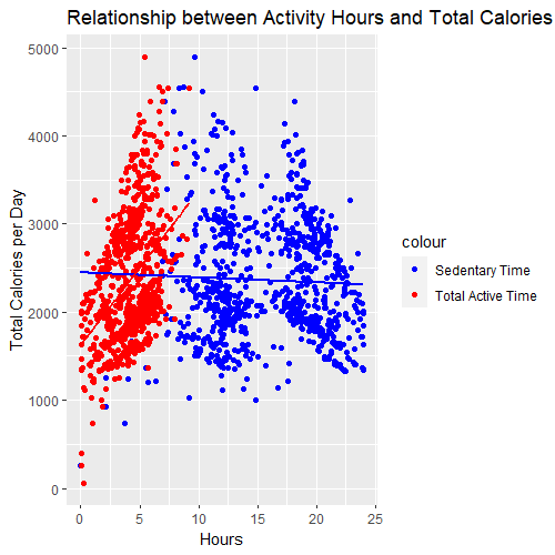
#Relationship between Activity Hours and Total Calories per Day
ggplot(merged_data, aes(y = calories)) +
  geom_point(aes(x = sedentary_hours, color = "Sedentary Time")) +
  geom_point(aes(x = total_active_hours, color = "Total Active Time")) +
  labs(x = "Hours", y = "Total Calories per Day", title="Relationship between Activity Hours and Total Calories per Day") +
  scale_color_manual(values = c("Sedentary Time" = "blue", "Total Active Time" = "red")) +
  geom_smooth(aes(x = sedentary_hours), color = "blue", method = "lm", se = FALSE) +
  geom_smooth(aes(x = total_active_hours), color = "red", method = "lm", se = FALSE)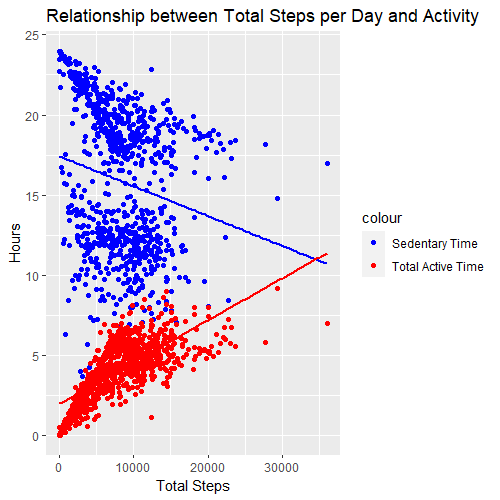
- As we were expecting there’s a positive correlation between the total steps taken and the total active time; and there’s a negative correlation between the total steps taken and hours doing sedentary activities.
- However, there are a few users that spend many sedentary hours but still manage to take a lot of steps, just like users who don’t spend many sedentary hours but don’t take as many steps as needed or expected. This suggests that other factors, such as intensity of activity or lifestyle, may influence step count beyond sedentary time alone.
- We have to remember that the sedentary hours include hours being asleep, so the negative correlation with the amount of calories burned we expected is almost nonexistent because different people sleep more or less and that’s counted towards sedentary time.
- As expected, there’s also a positive relationship between the total amount of calories burned and the total active time, but the negative correlation between the total amount of calories and the sedentary hours is very minimal; this can be attributed to the inclusion of sleep hours within sedentary time. Sleep duration varies among individuals and contributes to sedentary hours, which may weaken the negative correlation with calorie burn.
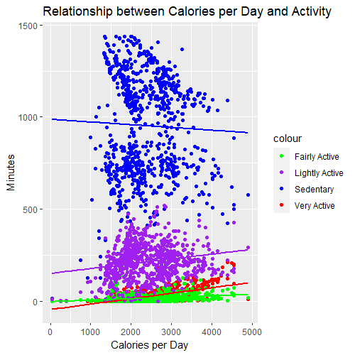
We can also plot by each category of activity time, for the number of total steps taken and calories burned.
#Relationship between Activity Time and Steps Taken per Day
ggplot(merged_data, aes(y = total_steps)) +
  geom_point(aes(x = sedentary_minutes, color = "Sedentary")) +
  geom_point(aes(x = very_active_minutes, color = "Very Active")) +
  geom_point(aes(x = fairly_active_minutes, color = "Fairly Active")) +
  geom_point(aes(x = lightly_active_minutes, color = "Lightly Active")) +
  labs(x = "Minutes", y = "Total Steps per Day", title="Relationship between Activity Time and Steps Taken per Day") +
  scale_color_manual(values = c("Sedentary" = "blue", "Very Active" = "red", "Fairly Active" = "green", "Lightly Active" = "purple")) +
  geom_smooth(aes(x = sedentary_minutes), color = "blue", method = "lm", se = FALSE) +
  geom_smooth(aes(x = very_active_minutes), color = "red", method = "lm", se = FALSE) +
  geom_smooth(aes(x = fairly_active_minutes), color = "green", method = "lm", se = FALSE) +
  geom_smooth(aes(x = lightly_active_minutes), color = "purple", method = "lm", se = FALSE)

#Relationship between Calories per Day and Activity Time
ggplot(merged_data, aes(x = calories)) +
  geom_point(aes(y = sedentary_minutes, color = "Sedentary")) +
  geom_point(aes(y = very_active_minutes, color = "Very Active")) +
  geom_point(aes(y = fairly_active_minutes, color = "Fairly Active")) +
  geom_point(aes(y = lightly_active_minutes, color = "Lightly Active")) +
  labs(x = "Calories per Day", y = "Minutes", title="Relationship between Calories per Day and Activity Time") +
  scale_color_manual(values = c("Sedentary" = "blue", "Very Active" = "red", "Fairly Active" = "green", "Lightly Active" = "purple")) +
  geom_smooth(aes(y = sedentary_minutes), color = "blue", method = "lm", se = FALSE) +
  geom_smooth(aes(y = very_active_minutes), color = "red", method = "lm", se = FALSE) +
  geom_smooth(aes(y = fairly_active_minutes), color = "green", method = "lm", se = FALSE) +
  geom_smooth(aes(y = lightly_active_minutes), color = "purple", method = "lm", se = FALSE)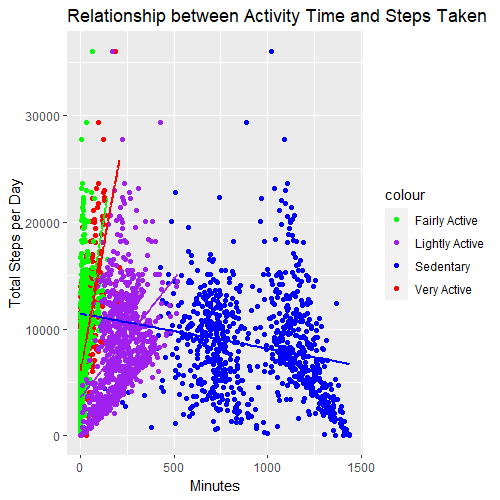
- For steps taken, the positive correlations are stronger for lighty active. This reinforces the idea that lightly active activities involve mainly walking. The relationship is less pronounced with fairly active activities and very active activities; this reinforces the idea that when these users do moderate and vigorous exercises, they mainly get involved in lifting weights and strength training exercises, rather than running or other cardio exercises.
- For the amount of calories, the correlations are in general the same but much less pronounced, especially for the sedentary time, which again might be because the sedentary time spend in our data includes time spend asleep.
Other Curious Findings
Let’s plot the relationship between steps and calories that are burned in a day, while also visualizing the number of sedentary hours spent in a day.
ggplot(data = daily_activity, aes(x = total_steps, y = calories)) +
  geom_point(aes(color = sedentary_hours)) +
  stat_smooth(method = lm) +
  scale_color_gradient(low = "darkblue", high = "lightblue") +
  labs(x = "Total Steps per Day", y = "Calories per Day", title = "Relationship between Steps and Calories per Day")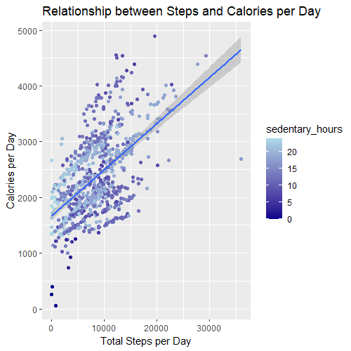
- Some users who don’t take many steps and engage in many sedentary activities are still burning a substantial number of calories (ranging from 1500 to 3000). In contrast, there are users who are more active and burn a similar amount of calories. This suggests that factors beyond step count and sedentary time, such as the intensity of activities and individual metabolism, can influence calorie expenditure.
Sleep Data and its Relationships
Now we’re going to analyze sleep data. First we want to know how many users have submitted this kind of data.
#Sleep Analysis
distinct_ids <- daily_sleep %>%
distinct(id) %>%
summarise(count = n_distinct(id))
distinct_ids$count
[1] 24
healthy_amount <- daily_sleep %>%
group_by(id) %>%
summarise(avg_amount = mean(hours_asleep)) %>%
filter(avg_amount >= 7 & avg_amount <= 9) %>%
summarise(count = n_distinct(id))
print(healthy_amount)
# A tibble: 1 × 1 count <int> 1 10
healthy_in_bed <- daily_sleep %>%
group_by(id) %>%
summarise(avg_time_taken = mean(time_taken_to_sleep)) %>%
filter(avg_time_taken <= 20) %>%
summarise(count = n_distinct(id))
print(healthy_in_bed)| # A tibble: 1 × 1 | |
| count | |
| <int> | |
| 1 8 |
- We only have sleep data for 24 FitBit users.
We want to know how many users, on average, sleep the recommended time of 7–9 hours.
- Only 10 users sleep the amount of hours recommended, which represents 43.48% of the users. This means that less than half the people are getting healthy recovering sleep.
We want to know how many users, on average, don’t take more to sleep than the recommended limit of 20 minutes.
- Only 8 users can fall asleep within the recommended maximum time of 20 minutes, which represents the third part of the FitBit users who submitted their sleep data. This tells us that most users have sleep difficulties and not very good sleep health.
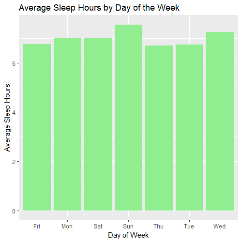
Let’s analyze the sleep time by day of the week, which can be analyzed by the total sum or the average; let’s analyze both.
#Total Sleep Hours by Day of the Week
options(scipen = 999)
ggplot(data = daily_sleep) +
  aes(x = day_of_week, y = hours_asleep) +
  geom_col(fill =  'darkgreen') +
  labs(x = 'Day of Week', y = 'Total Sleep Hours', title = 'Total Sleep Hours by Day of the Week')
ggsave('total_sleep_hours.png')

#With the average
avg_sleep_by_day <- daily_sleep %>%
  group_by(day_of_week) %>%
  summarise(avg_hours_asleep = mean(hours_asleep))

ggplot(data = avg_sleep_by_day) +
  aes(x = day_of_week, y = avg_hours_asleep) +
  geom_col(fill = 'lightgreen') +
  labs(x = 'Day of Week', y = 'Average Sleep Hours', title = 'Average Sleep Hours by Day of the Week')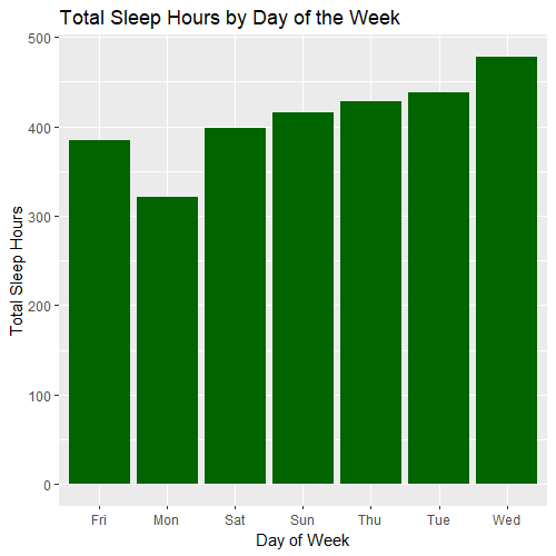
- Fitbit users sleep more time on Wednesdays and less on Mondays. We can see a pattern where users sleep less on Fridays, so they tend to sleep more on the weekends, but in Monday they sleep much less. This may be because on the weekends people have a different schedule in general, including for sleep; so people tend to sleep later and wake up later. This habit makes Mondays really tough for most people since they have to readjust to their original schedule, but their mind was used to the sleeping hours of the weekends, so it’s harder to fall asleep early so that people will sleep less on Mondays.
- Sundays and Wednesdays still exhibit higher sleep durations, aligning with the initial findings. It could indicate that individuals prioritize longer sleep on these specific days, potentially due to different schedules or lifestyle factors. For example, individuals may use Sundays to catch up on sleep after a busy week, while Wednesdays might be a mid-week rest day for some.
- Mondays may not necessarily reflect lower sleep duration on average, as initially observed. The revised analysis indicates that individuals, on average, may sleep longer on Mondays, possibly to compensate for sleep debt or to adjust to a new workweek.
- The initial observation mentioned that individuals tend to sleep less on Fridays. However, with the average sleep duration analysis, it’s not clear whether Fridays deviate significantly from the rest of the weekdays. This could imply that sleep duration on Fridays is more variable among individuals, with some maintaining their regular sleep routine and others staying up later due to the start of the weekend.
- Mondays and Fridays are more variable sleep days because of the start of the workweek and weekend. This supports the theory that most individuals have different sleep schedules during weekdays compared to weekends.
We can also analyze the sleep hours based on the average by the day of the week. Now Sundays and Wednesdays have more average sleep hours, and Mondays don’t exhibit such a drop. Here are my last explanations and conclusions:
Now, let’s see if there’s any correlation of the amount sleep with the amount of activity among users.
#Sleep Relationships
#The warnings we get are present because we did full outer joins so there will be a lot of null values in our merged data frame
ggplot(data = merged_data) +
  aes(x= hours_asleep, y = calories) +
  geom_point(color = 'red') +
  geom_smooth() +
  labs(x = 'Total Hours Asleep', y = 'Total Calories Burned', title = 'Calories Burned vs Hours Asleep')

ggplot(data = merged_data) +
  aes(x= hours_asleep, y = total_active_hours) +
  geom_point(color = 'orange') +
  geom_smooth() +
  labs(x = 'Total Hours Asleep', y = 'Total Active Hours', title = 'Total Active Hours vs Total Hours Asleep')

ggplot(data = merged_data) +
  aes(x= hours_asleep, y = total_steps) +
  geom_point(color = 'steelblue') +
  geom_smooth() +
  labs(x = 'Total Hours Asleep', y = 'Total Steps Taken', title = 'Total Steps Taken vs Total Hours Asleep')

ggplot(data = merged_data) +
  aes(x= hours_asleep, y = sedentary_hours) +
  geom_point(color = 'blue') +
  geom_smooth() +
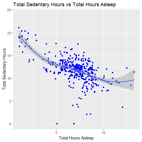
  labs(x = 'Total Hours Asleep', y = 'Total Sedentary Hours', title = 'Total Sedentary Hours vs Total Hours Asleep')

ggplot(data = daily_sleep) +
  aes(x= time_taken_to_sleep, y = total_minutes_asleep) +
  geom_point(color = 'steelblue') +
  geom_smooth() +
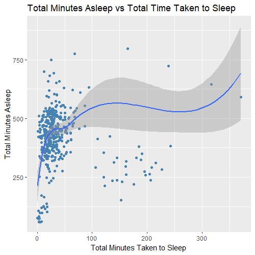
  labs(x = 'Total Minutes Taken to Sleep', y = 'Total Minutes Asleep', title = 'Total Minutes Asleep vs Total Time Taken to Sleep')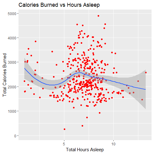
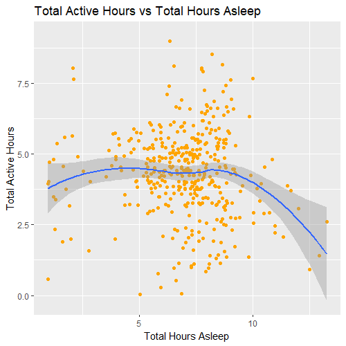
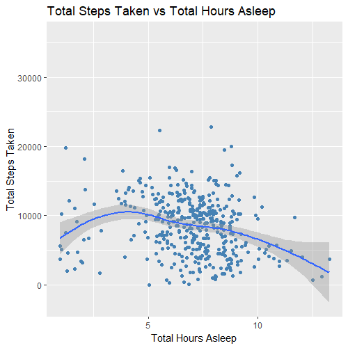
- There’s no correlation between the total hours people sleep and calories, total time being active or the total steps taken per day.
- There’s a negative correlation between the amount of time people sleep and the time they spend doing sedentary activities. This suggests that sleeping more makes people more energized and motivated to get involved in more active activities during the day.
- There’s a positive correlation between the time taken to fall sleep and the time being asleep, which means that FitBit users who take more time to fall asleep tend to have longer total sleep durations.
We can draw more conclusive insights from the sleep analysis:
- When comparing activity and sleep habits by day of week, we can conclude that users sleep more and do more physical activities during mid-weekdays Tuesdays, Wednesdays and Thursdays. This suggests that sleeping more contributes to having more energy and motivation to exercise during the day.
- Finally, we saw that users sleep more on Sundays, are less active but also don’t do many sedentary activities. This may be because Sundays is used as family day and day to relax doing activities outside, which are non-sedentary activities like going shopping, going to the zoo, among others. This reinforces the idea that sleep make people more energized and motivated to do activities outside even if it’s not exercise per se.
Summary of the Analysis
The data was formatted with dates in yyyy-mm-dd format, days of week in string format with the first three letters like ‘Sun’, date and time in the yyyy-mm-dd %H:%M:%S %p format, hours rounded to 2 decimals and percentages in 4 decimals. The data was filtered to records where the calories burned per day or the total active hours are less than or equal to 0.
All the tables were organized by “id” and the “date”, and also by “hour” for the tables that include time information. The data then was merged using joins. A merged data table that peforms a full outer join on the three main tables daily_activity, weight_log and daily_sleep, joined by “id” and “dates”. An hourly data table that performs a full outer join for the 3 main tables that have time information hourly_calories, hourly_steps and weight_log, joined by “id”, “dates” and “hour”. When analyzing days of the week, the data table was organized with the days numbered from Sunday=1 to Saturday=7, sorted in ascending order.
Insights and trends that were discovered from the analysis:
- Bellabeat customers mainly record and track their activity, steps, calories and sleep information, they don’t often keep track of their weight or water intake.
- There’s weight data for only 27% of users, because most of them find issues and have to submit the weight data manually, which discourages them to use this feature.
- As expected, increased physical activity, measured by active hours and step count, is associated with higher calorie burn.
- The relationship between sedentary hours and calorie burn is influenced by sleep duration and other factors, leading to a weaker correlation.
- There is a negative correlation between the total steps taken and hours spent in sedentary activities. However, some users defy this pattern, with some spending significant sedentary hours but still managing to take a considerable number of steps. And others who spend fewer sedentary hours but do not meet the expected step count.
- The relationship between intensity activities and steps taken is stronger for lightly activities compared to moderate and vigorous activities.
- Some users who don’t take many steps and engage in significant sedentary activities still burn a substantial number of calories.
- Users are active on approximately half of the days within the entire month. Only 26.67% of users manage to do moderate or vigorous exercise for the recommended quota of 22 days.
- Users are more active on mid-weekdays from Tuesdays to Thursdays, but also spend more time in sedentary activities these days. Users are less active on Sundays, but also spend less time in sedentary activities.
- Users cover more miles when they’re lightly active, and less with moderately-intensity activities.
- Most users don’t get enough sleep and take long to sleep.
- Users sleep more on Sundays and mid-weekdays Tuesdays, Wednesdays and Thursdays. Mondays and Fridays are more variable sleep days because of the start of the workweek and weekend.
- There’s a negative correlation between the amount of time people sleep and the time they spend doing sedentary activities.
- There’s a positive correlation between the time taken to fall sleep and the time being asleep.
- Users sleep more and do more physical activities during mid-weekdays Tuesdays, Wednesdays and Thursdays.
- Users wake up later on the weekends.
- Users sleep more on Sundays, are less active but also don’t do many sedentary activities.
- Users tend to take the most naps on weekends, with Wednesdays and Tuesdays also showing a relatively higher frequency. In contrast, fewer naps are observed on Mondays and Fridays.
These insights help to answer the business question because they provide us with ways on how customers are using Bellabeat products. Consumers use more the Leaf and Time Bellabeat products, along with the Bellabeat app, since they’re more interested in tracking activity, steps, health and sleep habits.
They also help us understand relationships between physical activity, sedentary behavior and calorie burn, as well as activity and sleep patterns, so we can identify targeted audiences, product development opportunities, personalized recommendations and streamlining marketing content.
Presentation and Dashboard
Bellabeat Data Analytics Case Study Tableau Dashboard:
https://public.tableau.com/views/DataAnalyticsCaseStudy-Bellabeat/Dashboard1?:language=en-US&:display_count=n&:origin=viz_share_link
Bellabeat’s Smart Device Usage and Health Trends Presentation:
https://docs.google.com/presentation/d/e/2PACX-1vQAjU1ADV-L6ol1YbUeNoUOeAYDa4l2-zM3jsB4ckMVTnMMNLN8QW3h9TS7zC87Xw/pub?start=false&loop=false&delayms=3000
Jaime A. Velasquez’s Portfolio — GitHub Repository:
https://github.com/jaimeandrevelasquez/jaimeandrevelasquez.github.io
ACT PHASE
Conclusions
- Bellabeat customers mainly use the Leaf and Time Bellabeat products, along with the Bellabeat app.
- Regular physical activity and walking are very important for overall calorie/energy expenditure.
- Factors beyond sedentary time, such as activity intensity or lifestyle, influence step count.
- There are recording issues with weight data, therefore most users don’t use this feature.
- Light activities primarily involve walking, while moderate and vigorous activities mainly involve lifting weights and strength training.
- Factors beyond step count and sedentary time, such as activity intensity and individual metabolism, influence calorie expenditure.
- Most users need to do more physical activity to be healthy and a few healthy users are exceeding their exercise time.
- The intensity of the activities influences step count and calorie expenditure.
- Despite work and school activities, users prioritize doing physical activities during mid-weekdays Tuesdays, Wednesdays and Thursdays; this means that users are more motivated and energized to do physical activities in the middle of the week.
- On Sundays, most users prefer to relax in non-sedentary activities like recreational activities outside.
- Most users are sleep deprived and don’t have a good sleep hygiene.
- Sundays serve as a recovery day after a busy week, while Wednesdays offer mid-week rest opportunities.
- Users have different sleep schedules during weekdays compared to weekends.
- Users with longer sleep onset times experience deeper and more consolidated sleep once they do fall asleep.
- Sleeping more makes people more energized and motivated to do more physical activities during the day.
- Naps help people rest and recover to be more active during the day but they’re taken mostly the days when users have more free time.
Recommendations
- Bellabeat product improvements: The Bellabeat app should encourage people to engage in physical activities by vibrating or emitting sound when it detects that the user has been sedentary for a personalized healthy limit. Bellabeat should also add more functionalities like measuring the quality of sleep, body temperature, blood pressure, brain activity and biochemicals released, and address issues like weight recording.
- Implement an incentive system: Bellabeat should set personalized healthy milestones and reward their users when they hit their weekly milestones and when they complete challenges. This will incentivize their members to achieve their health goals by getting discounts for Bellabeat products and memberships that offer exclusive content. The app algorithm should provide tailored limits and suggestions for optimizing activity levels, managing sleep routines, and achieving individual goals.
- Address mid-week motivation and weekend wellness focus: Bellabeat should develop content and promotions that align with users’ behaviors during the week, like targeted challenges, milestones and rewards at midweek to encourage users to maintain their motivation and engagement during these days; as well as weekend challenges and tailored workout plans to gain energy and momentum to start exercising, and sleep-aid material to help maintain their sleep schedule on the weekends.
- Targeted marketing campaign for two segments: Bellabeat should target its marketing campaign for two distinct segments. The first comprises individuals who are already health-conscious and engaged in fitness activities, but want to optimize their performance and overall health. For this segment Bellabeat should position its products and app as the ultimate fitness companion, offering comprehensive tracking and motivation for exercise, steps, calories, and sleep health so that they can achieve their best performance and healthy lifestyle goals. However, Bellabeat should also enhance awareness regarding the significance of weight and hydration tracking as essential elements for overall well-being.
The other segment consists of individuals who have the desire to improve their overall health but haven’t been successful. To target this larger potential market, Bellabeat should highlight the transformative benefits of their products and showcasing how Bellabeat can support individuals in their wellness journey. - Partnerships and education: Bellabeat should partner with health and wellness experts and brands to collaborate in aiming to educate people on best practices and routines for improving their health, and managing health issues by conducting free webinars, workshops, online sessions and publishing articles on social media.
Further Exploration:
- Obtain data from many more users and for a longer time frame like at least one year for a more comprehensive, accurate analysis and to answer the question: What are some monthly trends in Bellabeat smart device usage?
- Obtain data for the Spring product to answer the question: What are some trends in Spring usage and hydration patterns?
- Track the behavior change patterns of Bellabeat users over an extended period to identify sustained engagement, behavior modifications, and long-term impacts of using Bellabeat products on users’ health and well-being.
- Conduct user surveys and feedback analysis to understand their experiences and satisfaction with Bellabeat products and the app.
And that’s the end of our Data Analytics Case Study! Thank you for reading, I hope you’ve found it interesting, useful and inspiring.

Comments
Post a Comment